
Forecasting using a combination of quantitative methods and your own experience as a demand planner is what will set you apart in your industry.
Overview of Exponential Smoothing
Like the naïve and moving averages methods, exponential smoothing uses historical demand data to forecast. Although this demand forecasting method is a little more complicated, it provides some distinct advantages over the two simpler methods.
Benefits
One of the benefits of this model is that it takes the most recent observations into account and weights them accordingly. For example, if we are looking at four years of demand forecasts, April/May/June of 2014 will likely be weighted differently in April/May/June of 2019. The exponential smoothing method takes this into account and enables us to plan inventory more efficiently by placing greater weight on more relevant, recent data.
Another benefit is that spikes in the data aren’t quite as detrimental to the forecast. In exponential smoothing, the most recent forecast has the greatest weight and therefore should be the most accurate in predicting demand, as opposed to the moving averages method where the weight for each period is fixed.
Limitations
While these advantages are great when planning inventory for a specific month, the exponential smoothing model limits our ability to forecast demand using seasonality. This model also cannot be used to identify trends.
Although these limitations are inconvenient, this model helps us establish a nice foundation for more complex demand forecasting models. Let’s get into it!
How Does Exponential Smoothing Work?
To understand this forecasting model, let’s look at an example using a 4-year historical data set.
Because this method requires demand planning expertise, you, as the demand planner, are going to have to choose a value for what is known as the “smoothing constant.” This constant will determine the impact that prior observations have on the forecast. In our forecasting equation, we will represent the constant as α.
The equation for exponential smoothing is
Forecast for period 1 + α*(Actual Sales for period 1 – Forecast for period 1)
The best way to identify your smoothing constant is to understand the difference between a high decimal and low decimal. The smoothing constant is going to be a number between 0 and 1.
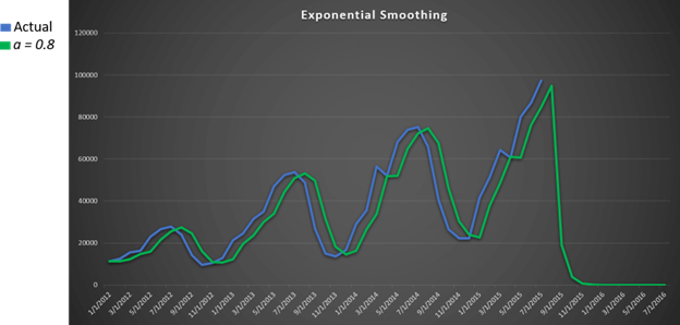
The higher a smoothing constant, the more sensitive your demand forecast. This means you will see large spikes of data. This is what a smoothing constant of 0.8 would look like with our data set:
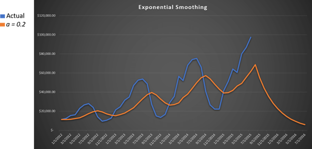
The lower a smoothing constant, the less sensitive the forecast and thus the smaller and/or fewer the spikes in demand the forecast will show. This is what a smoothing constant of 0.2 would look like with our data:
Formula:
Knowing what smoothing constant to use is an important part of demand planning. To determine your smoothing constant, you need to know your company, your products, and your inventory.
If you’re just starting out, there is a trial and error method you can use to determine the best smoothing constant for your situation:
- Create four columns of possible constants, e.g. 0.2, 0.4, 0.6, and 0.8., next to your original data set.
- View all five on a graph and determine which constant, or which combination of constants, best fits.
How Does Exponential Smoothing Apply to Inventory Planning?
Forecasting using a combination of quantitative methods and your own experience as a demand planner is what will set you apart in your industry. If you know that your product typically tends to have a high level of noise, then you should plan to use a small constant. If you know your product has a low level of noise, it would make sense to use a higher constant, because you won’t have to worry about data spikes too often. Understanding how to best use exponential smoothing for your company’s circumstances will facilitate accurate inventory tracking and good decision making.